Education is an investment. After investing time, effort, and money, one’s value increases, hopefully in such a way that also translates to higher pay. Here we show that a community that shares in the cost of an individual’s education, will also later share in its value. What follows is a simple network model that clarifies and quantitatively supports this contention.
Value and the Success Index
We define one’s value, vᵢ, as not only an individual’s net worth, but also his or her expertise, time, skills, assets, and so on.Note: When discussing value in the abstract, we refer to this abstract definition that includes everything one can offer in a transaction, but in our simulations, we treat value as one’s net worth, since that is easier to approximate and the results are then more immediately interpretable. Nevertheless, the same results hold (in a qualitative sense) for the more abstract notion of value, as defined above.An individual’s value, however, is not all the value to which one has access. For example, while Bill Gates’ net worth is $130B, with friends like Warren Buffett, he has access to much more wealth than that. We therefore define one’s success index, sᵢ, as one’s own value plus some fraction of the value of one’s connections. This not only includes one’s immediate connections, but also second, third and fourth degree connections, since these are usually also accessible (although with farther connections, one has access to an even smaller fraction of their value). Mathematically, we can write this as follows:
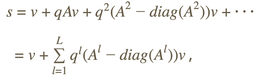
where, for a community of size N, s is the vector of the success indices of each of its members, i.e., s=(s₁,..., sᵢ,..., sₙ); v is the same sized vector of the individual values of each member, q ∈ (0,1) is the average fraction of value an immediate neighbor would be willing to share; A is the adjacency matrix (an N × N matrix whose (i,j) th element is 1 if individuals i and j are connected, and 0 otherwise); L is highest degree of connections one may have access to (we have set L=4 in the simulations); and diag(•) is an operator that, for any square matrix, returns the same matrix but all non-diagonal entries equal to zero.
Model and simulations setup
The initial network was set up with N₀=100 individuals, each of whom was given a value drawn from an exponential distribution with a scale parameter of 1×10⁶. Each value in the N₀×N₀ adjacency matrix A₀ for this initial community is drawn from a binomial B(1,0.1). For the kth additional node that is added to the community, we draw an (N₀+k)-dimensional column vector b, also from B(1,0.1), and obtain Aₖ by concatenating b with Aₖ₋₁ horizontally, and its transpose bᵀ vertically (with a 0 along the diagonal). Thus, for every k, Aₖ is the adjacency matrix for the entire network, including the k individuals added. The value of every individual added was initially sampled from an exponential distribution with a scale parameter of 1×10⁴. We then distinguished three groups:
Null: Individuals whose value stays constant. This serves either as a model for those not pursuing further education, whose value is not, on average, expected to increase as substantially; or as a standard relative to which we compare the evolution of the other two groups.
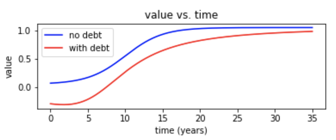
Without KHS: This is a group that incurs debt for their education, with a resulting delay in the trajectory of the growth of their value.
With KHS: This is the group whose debt is fully or partially paid off, i.e., the beneficiaries of KHS.
The following figure shows the sigmoidal growth curves for the second and third groups, with the value measured as a fraction of the individual theoretical maximum value.
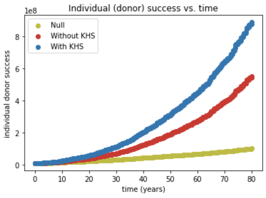
The average success for the entire community was measured after the addition of each new member. We also tracked the success of one of the members of the original community (a “donor”), and of one of the members that joined later (a “joiner”). Finally, we reported the distribution of success indices for each of the three groups as a function of the number of individuals added.
Results
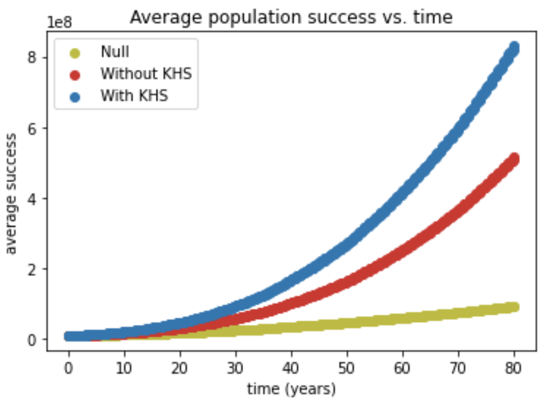
Below we present figures displaying the results of adding 800 individuals to a network initially consisting of 100 individuals. The rest of the parameters are as outlined above. Success is measured as a function of individuals added. When time is indicated (in years) this is assuming 10 individuals are added a year.
As the figures below show, not only is the average success of the entire community growing much faster under the KHS model, but even donors and joiners experience the same kind of growth on an individual level.

Below is the distribution of success over three same-sized populations as a function of the number of joiners (s(0)is the distribution of the initial N0=100 individuals, which is identical for the three groups). The average of each distribution grows according to the figures above. The red and blue distributions have a wider spread presumably because joiners are at different points in their value growth curve (see the figure in the previous section).
To obtain the code for the simulations, please feel free to reach out to Daniel at daniel@kochvei.org.